Parallelisation Strategy
PDAF can be run both in serial and parallel.
In either cases, Message Parsing Interface (MPI) is used.
In (py)PDAF, users need to specify the MPI communicators for the model (comm_model),
the filter(comm_filter), and the coupling (comm_couple)
between the model and the filter. These communicators are specified when PDAF is initialised
by pyPDAF.PDAF.init.
In MPI, a communicator is formed by a group of processes.
The default communicator in MPI is called MPI_COMM_WORLD.
If we design a program run by npes_world = 12 processes,
the default MPI communicator, MPI_COMM_WORLD, controls all these processes.
In (py)PDAF, one can make use of all processes,
or only a handful of these processes.
In the former case, the communicator for an ensemble system
is comm_ens = MPI_COMM_WORLD with npes_ens = 12 processes.
In the latter case, one can choose a few processors (npes_ens)
as communicator comm_ens dedicated to PDAF, and the rest processors
can be used for other tasks, e.g. I/O operations.
The MPI communicator used by (py)PDAF can be set
by pyPDAF.PDAF.set_comm_pdaf.
Online mode

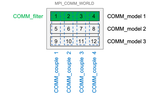
Here is an illustration of the parallel strategy for an online DA system.
The example in this figure uses npes_ens = 12 with npes_model = npes_filter = 4
where the filtering (filter commnicator) is done on one of the model communicators.
The model is decomposed into 4 sub-domains in this figure. Each coupling communicator
collects state vector from each model process running the same model domain.
Model communicator
Here, comm_ens can be divided into 3 model communicators (model_comm),
each of which has npes_model = 4 processes.
In the context of PDAF, each model communicator can perform an independent model run.
That is, we have 3 parallel model tasks (n_modeltasks = 3). In this specific example,
if we have 3 ensemble members (
dim_ens = 3), each model task runs one ensemble member. This is the case in the figure above. This means that the ensemble members local to the model task,dim_ens_l = 1. This setup is calledfully flexiblesetup in PDAF.in the case that
dim_ens > 3, each model task runs more than one ensemble member serially. Each model task could also have different number of local ensemble members asdim_ensis not necessarily a multiple ofn_modeltasks. For example, ifdim_ens = 4, one model task runsdim_ens_l = 2ensemble members serially and others just runsdim_ens_l = 1ensemble member.
Filter communicator
In our example, one model task runs on npes_model = 4 processes.
For the sake of efficiency, most physical climate models perform domain decomposition.
Under the domain decomposition, the model domain is divided into smaller domains,
and each process only simulates a sub-domain. To make the example more concrete,
if the model has 2 variables and 44 grid points, each sub-domain will
simulate 11 grid points. The model domain decomposition fits well with the
concept of domain localisation where the filtering algorithm perform assimilation
for each element of the state vector individually, e.g.:
for element in state_vector:
    do_assimilation(element)
The domain localisation is great for parallelisation as the assimilation of each element of the state vector is completely independent of each other. In (py)PDAF, one can follow the domain decomposition of the model. In this case, one of the model communicators can be used as a filter communicator (comm_filter) where the number of processes performing filtering is npes_filter = npes_filter = 4. In the example above, each local domain contains dim_p = \(2 \times 11\) number of elements in the process-local state vector, state_p, where the subscript p represents arrays on a specific process, or PE-local. Certainly, this means other model communicators are not in use during the filtering stage, but it is a good compromise compared to the increased complexity of redistributing the state vector.
Coupling communicator
In the filtering stage, ensemble systems must gather model state from each ensemble member to the filtering processes. This is done by a coupling communicator (comm_couple), where model processors simulating the same sub-domain are grouped together. The number of processes used for coupling is usually n_modeltasks. After the filtering, the coupling communicator is used to distribute the analysis back to the model for following simulations.
Offline mode
In PDAF, the parallelisation of the offline mode is a simplification of the online mode. In offline mode, the DA program only performs the filtering algorithm. If the filtering is performed in serial, the model, filter and coupling communicator are all given as comm_ens with npes_ens = 1.

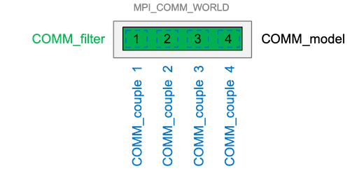
Here is an illustration of the parallel strategy for an offline DA system. The example in this figure uses npes_ens = 4 with npes_model = npes_filter = 4. The model is assumed to be decomposed into 4 sub-domains in this figure.
For the filtering algorithm supporting parallelisation, if npes_ens = 4, the state vector is partitioned into npes_model = npes_filter = 4 state vectors that is local to one process, state_p, where the subscript p represents process-local, or PE-local. This means that each process performs filtering for only a section of the full state vector, and PDAF assumes that the ensemble model is run by npes_model = 4 number of processes. The reason for this treatment is explained in Filter communicator setup in online mode. In this case, comm_filter = comm_model = comm_ens. The coupling communicator is used to collect ensemble from different model tasks to the filter processes in online mode. In the offline mode, the model state is read from disk files, and only one model task is run. Hence, one comm_couple corresponds to just one model process.